River level forecasting
In this article I explore an approach to producing free forecasts of river level heights for the river Cam (the main river in Cambridge). I will discuss the process of finding and storing the data and discuss different ways to produce the forecasts. Lastly, we implement this in production so it can be accessed by potential users. All of this was done using free software / sites.
This is intended to be a helpful guide to implementing a similar forecasting measure on other rivers.
Motivation
While studying in Cambridge, I was involved in college rowing as a rower and a cox. Outings were often cancelled due to poor weather conditions and this usually happened with relatively short notice. Rowing on the Cam (Specifically on the section between Jesus Lock and Baitsbite Lock) is governed by the CUCBC (Cambridge University Combined Boat Clubs). Outings are typically cancelled due to something called the flag which is set to different colours depending on how safe it is to go out on that day. Typically, conditions that lead to an outing being cancelled are:
- High wind speeds (35mph or so)
- Fog / Mist leading to poor visibility
- Extreme cold
- High water levels or fast flowing water The first three of these can usually be determined in advance by weather forecasts but the last one, the river height and current speed, is not easily obtainable. It’s also one of the more common reasons for cancellations.
River
Data sources
To be able to do any forecasts, we of course need data. To ingest data from different sources, one viable method is to use google sheets. This online spreadsheet system has several useful functions we will use to automate the ingestion of data. I set up a system of google sheets that collected river information hourly and then after letting this run for a few months I performed the analyses. This was primarily because for some of the sources there was no way to download historical data, only current data.
Data availability
Another important consideration is when data is available. Checking the UK government hydrology data explorer found here we can see three recording stations upstream of the centre of Cambridge that could be useful:
- Burnt Mill - River Rhee
- Stapleford - River Granta
- Dernford - River Cam However, the only way to obtain measurement values from these stations has a time lag of approximately 2 days. One can determine the width of the river at the monitoring station using the NRFA (National River Flow Archive) site, for instance for the river Granta we can access rough size estimates and pictures. Using these as well as typical river heights from the government hydrology site we can determine rough estimates of the cross sectional area of the rivers. We can also get river flow volume data from the nrfa and hence determine the river speed (roughly). Doing so and using google maps to estimate the distances, one can find that the water would flow between the station and the portion of the Cam we’re concerned about in between 6 and 24 hours, so the two day time lag makes this information useless for forecasting as it is available too late.
River levels
For the portion of the Cam where rowing takes place, there are three nearby stations for which data could be relevant for forecasting and d One good site to consider for obtaining river height data across England, Scotland and Wales is riverlevels.uk which displays data for all river level monitoring stations. For the portion of the Cam that rowing outings usually take place on, the relevant monitoring station is the Jesus Lock Sluice Auto Cambridge Monitoring Station, which can be found here. River levels UK only displays the current value on the site, however past values can be downloaded in the form of a csv. To import this in sheets we use the sheets function:
=IMPORTXML("https://riverlevels.uk/jesus-lock-sluice-auto-cambridge-cambridgeshire","/html/body/div[4]/div[1]/div/div[1]/h2/span")
The first entry is the link to the website, and the second entry is the XML path to the part of the webpage that contains the river level value. One can determine this path more generally by using inspect element, then finding the html code corresponding to that part of the website. Next, one can right click on this portion and click “Copy XML path” to get the “html/body/div…” code for that component of the webpage.
There are other parts of the river we also want to collect data for. These are the height just above Jesus Lock, and just below Baitsbite Lock. The sluices above stream are adjusted to keep the height approximately the same, but the small variations may still have explanatory power. We get these data sources directly from the government Hydrology API. In the sheets implementation we import this data using code like:
=IMPORTDATA("http://environment.data.gov.uk/flood-monitoring/id/measures/E60501-level-stage-i-15_min-mASD/readings?latest")
This gets the most recent value as a JSON file which then spans multiple cells in Google Sheets. We’re concerned with the value of that monitoring station, which can be found several lines into the JSON file we import. If one wants to look at more data, then they can write into a cell in sheets:
=IMPORTDATA("https://environment.data.gov.uk/flood-monitoring/id/measures/E60502-level-downstage-i-15_min-mAOD/readings?_sorted&_limit=2200")
And then we can change the _limit parameter to vary how many records are shown. One can then reorder and transform this data to get the most recent n samples from that monitoring station. For my sheets implementation I only used the most recent values so this was not needed, but for another project it may be helpful to go back into the past using a large _limit value.
I then put all of these into a single row in sheets, with columns:
- Date
- Time
- Flag (the colour of the flag at that time)
- Height (Just below Jesus Lock)
- Above JL Height (Height just above Jesus Lock)
- Baitsbite Height (Height just below Baitsbite Lock)
This row updates live, and changes every hour. We want to store this data, which can be done by using Apps Script to automatically record the data hourly. I set up a trigger that runs every hour, and on the trigger it runs the following function (written in TypeScript):
function record_data(){
  var Daily_data = SpreadsheetApp.getActive().getSheetByName("Hourly data")
  var data_range = Daily_data.getRange(2,1,15,10).getDisplayValues()
  var Records = SpreadsheetApp.getActive().getSheetByName("Records")
  for (let i=0; i < data_range.length; i++){
    Records.appendRow(data_range[i])
  }
}
This copies the line the hourly updated data is on in the Hourly data sheet to the bottom of the Records sheet. For other projects where you have different amounts of data, the same approach will work but you may need to get a different range in the Daily_data.getRange(2,1,15,10) part of the code.
Historical Weather data
There are several options for weather sources. I opted to use the Cambridge computer lab’s raw daily weather data, which can be found here. This source was chosen because of it’s low latency. One can get the data for Monday on Tuesday just after midnight. One can also obtain the current weather conditions on a different page found here. Other sources generally had some small time lag that made them less useful for short term forecasting. We will now discuss the data provided by this source. Data is stored as text files for each day, and has the following columns:
- Time
- Temp - Temperature (in degrees celsius)
- Humid - Humidity (in % from 0 to 100)
- DewPt - Dew Point (in degrees celsius)
- Press - Pressure (in milibars)
- WindSp - Wind speed (in knots)
- WindDr - Wind direction (takes values like “N” for north)
- Sun - Cumulative number of hours of sum (values in [0,24])
- Rain - Cumulative amount of rainfall (in milimeters) (One should note that in some files it is cumulative, and in others it is not)
- Start - Start time of the recording for that day (time, e.g. 00:00)
- MxWSpd - Maximum wind speed (in knots) Of these, domain experience can tell us that the only column that may be relevant for forecasting the river level is the cumulative amount of rainfall. If one wished instead to create predictions of the river flag colour then the Humidity, Wind speed and Max wind speed may also be relevant.
Importing the Weather data
One approach is to import the current data using:
=IMPORTDATA("https://www.cl.cam.ac.uk/weather/txt/weather.txt")
And add it as an extra column on our sheet to be recorded daily. The data from this source has cumulative rainfall, so if we store the cumulative rainfall, we can compute the rainfall in the past hour by subtracting the rainfall up to the previous hour (which has already been recorded) from the current rainfall.
Looking around the Computer Lab site we can also see the option to download the historical data since 1995 as a csv from the site and then transform this data into our desired output in sheets. The Computer Lab data is half hourly, so we will sum the rainfall to get the total amount each hour. Something like this could be used to fill in past data if all of your data sources provide historical data.
Accessing the data
As described above, the system imports the relevant data into a google sheets file that uses automated triggers to store the new data as it comes in. In the Github repository one can see a data file, which contains a csv that updates automatically using Github workflows. To access the data, one can use any way to import a csv hosted on Github. For instance using Pandas in Python:
url = "https://github.com/ScottHislop/RiverHeightPredictions/blob/main/data/river-data.csv?raw=True"
river_data = pd.read_csv(url)
or for R, one can use:
url <- "https://github.com/ScottHislop/RiverHeightPredictions/blob/main/data/river-data.csv?raw=True"
river_data = read.csv(url)
If you want to use exactly the same data as I did below, download this csv
Exploratory Analysis
We will now explore our data and determine a good model for our data. I chose to use the language R for this, as it has some powerful time series analysis packages. We’ll be using the package fpp3 for most of our analysis, which is based on a book Forecasting: principles and practice, 3rd Edition. Firstly, we read the csv from the Github and convert it to a tsibble using the following code:
url <- "https://github.com/ScottHislop/RiverHeightPredictions/blob/main/data/river-data.csv?raw=True"
river_data <- readr::read_csv(url)

river_data <- river_data|>
  mutate(Hour = dmy_hms(Datetime))|>
  select(-Date,-Time, -Datetime, -Flag)|>
  as_tsibble(index=Hour)
Next, we perform a test-train split on our data, putting the first 2000 data points into the train set, and the rest into the test set. We then produce a plot of the height over time using the following code:
ggplot(train_river_data,aes(x=Hour))+
  geom_line(aes(y=Height, color=as.factor(Flag)))+
  geom_line(aes(y=Rain/15+3.8))+
  scale_y_continuous(
    "River Height at Jesus Lock",
    sec.axis = sec_axis(~(.-3.8)*15, name="Rainfall (mm)")
  )+
  scale_color_manual(name="Flag", values = flag_color_vec)+
  xlab("Time")+
  ylab("Jesus Lock Sluice Height")
Where flag_color_vec is a vector describing which colours different flags should be coloured in as on the plot. We also plot the rainfall, changing the axes so they match up for easier interpretation. This produces the following:
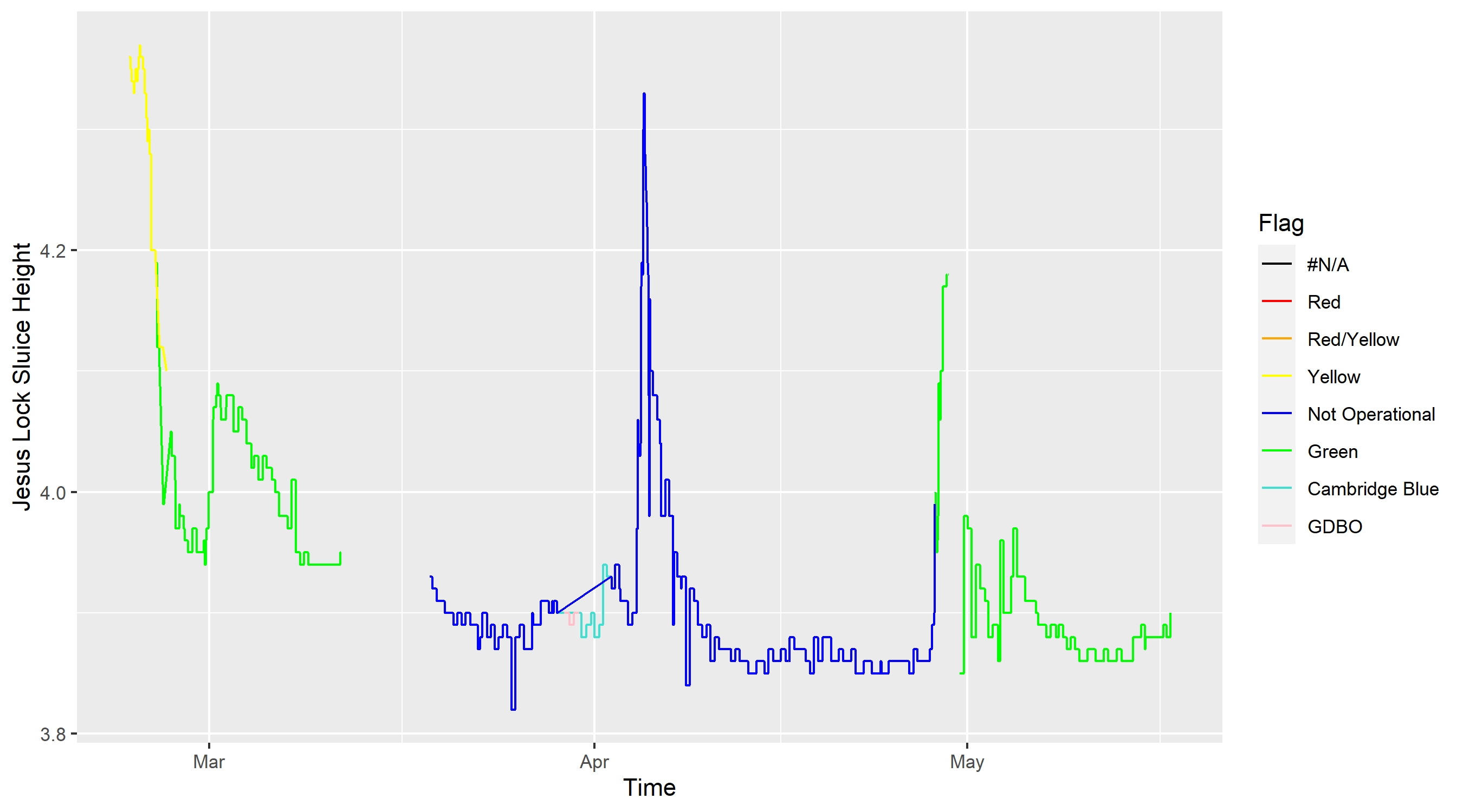
There are several interesting points to note here, both about the data quality and the river heights:
- River heights seem to be between 3.8 meters and 4.2 meters high most of the time (Note that this height is not necessarily the depth of the river and we mostly care about relative changes in height)
- Cancellations tend to happen when the height goes above 4.2m, although there is some variation
- Outings are generally trickier (in the sense that inexperienced coxes are likely to struggle) when the height is above 4.1m. This is also when banks are likely to be flooded. These rare events are the ones we care most about.
- There are some portions of the data with NA values. This was the result of riverlevels.uk changing where on the site they store the data. One could fix this by downloading the csv and filling in the gaps.
- Rainfall definitely seems correlated with the river height, but some time periods (mid April) have large amounts of rainfall with no increase in river height, while other periods (early April) have a similar amount of rainfall and a large increase in river height.
Explanatory variables
We have 3 explanatory variables:
- River height just upstream of Jesus lock
- River height just below Baitsbite lock
- Rainfall
We would not necessarily expect rainfall to be particularly correlated with river height. This is because it takes some time for rain to flow into the portion of the river we have data for. Hence, if we saw a high spike in rainfall we might expect river height to increase a few hours later. Also, one can see that medium strength rainfall for a few hours would lead to similar changes in river height to a single hour of very strong rainfall. For this reason, a model considering lags in the relationships is needed.
For the other variables, the river heights above and below the portion of the river we’re concerned with, it is plausible that they have some effect on the current height and furthermore that this effect is near instantaneous. This is because the Sluice’s that manage the height of the Cam and ensure the upstream height is kept low enough to prevent flooding have access to the data near instantly, so the rates of flow into and out of the section of river we wish to forecast may well be instantaneously affected by the explanatory variables. For this reason, we show the correlations between them:

This is a plot created using the R function:
GGally::ggpairs()
On the top right, we see correlation values between the two variables. On the bottom left, we see scatter plots of the two variables against one another. The diagonal contains density plots of the three variables. From this collection of plots, we see that the correlation between the above JL height and the height is particularly strong (as we would predict from the previous paragraph). We also see that the above JL height seems close to normally distributed, while the other heights have fat right tails. This is likely because the upstream height is kept as close as possible to constant to enable punters to use that section of river, while when heavy rainfalls occur the regions below Jesus Lock and below Baitsbite Lock tend to flood fairly heavily.
Models
Linear model
The first model we consider is perhaps the most basic, and will be used for comparison to other, more complex (and hopefully better performing) models. We will fit a linear model with dependent variable height, and independent variable rainfall. Doing so using the R code:
train_river_data|>
  model(TSLM(Height ~ Rain))|>
  report()
One finds the output:
Series: Height
Model: TSLM

Residuals:
     Min       1Q   Median       3Q      Max
-0.10989 -0.05989 -0.03961  0.02011  0.44011

Coefficients:
             Estimate Std. Error  t value Pr(>|t|)
(Intercept)  3.929885   0.002338 1680.526   <2e-16 ***
Rain        -0.018031   0.007297   -2.471   0.0136 *
---
Signif. codes:  0 ‘***’ 0.001 ‘**’ 0.01 ‘*’ 0.05 ‘.’ 0.1 ‘ ’ 1

Residual standard error: 0.09757 on 1806 degrees of freedom
Multiple R-squared: 0.00337,	Adjusted R-squared: 0.002818
F-statistic: 6.106 on 1 and 1806 DF, p-value: 0.01356
From this we see:
- Our residuals do not seem to be normally distributed, or at least the quantiles suggest the fit is far from perfect
- The OLS estimate of the Rainfall coefficient has a negative value, implying rainfall actually reduces river height. It is also statistically significant.
- The R squared value and adjusted R squared value are both very low, but we cannot yet determine if this is due to noisiness in our data or poor model performance.
One can also look at the time series residuals plot:

We can clearly see the model doesn’t fit our data well as one should see:
- No pattern in the innovation residuals (We see clear evidence of patterns)
- Few (if any) points in the ACF plot outside of the Ljung-Box lines (Our model has every single value outside of the lines, implying strong autocorrelation between the residuals)
- Normally distributed residuals (ours clearly have a very strong right tail)
Dynamic regression
This is a technique which extends the linear model from the previous section. Instead of using iid normal random variables as the errors in our model, we let the errors contain autocorrelation. More specifically, we have:
\[y_t = b_0 + b_1 x_{1,t} + n_t\]where $n_t$ is some ARIMA model. The model then has two error terms, one from the regression model ($n_t$) and another from the ARIMA model. We assume the errors in the ARIMA model are white noise. Note that the model estimates are generally invalid when the data is non stationary. When time series are non stationary then we could employ differencing (Using $y_t - y_{t-1}$ instead of $y_t$) to remove the non stationarity and then fit the model on the differenced time series. One can automatically fit the best type of ARIMA model using the following code:
fit_dyn_reg <- train_river_data|>
  model(ARIMA(Height~Rain))
One can then see the model fitted using report() and find:
Series: Height
Model: LM w/ ARIMA(0,1,0)(1,0,0)[24] errors

Coefficients:
        sar1    Rain
      0.0142  -6e-04
s.e.  0.0249   9e-04

sigma^2 estimated as 0.0001514:  log likelihood=5280.6
AIC=-10555.2   AICc=-10555.19   BIC=-10538.38
Close inspection of this model reveals that it has automatically selected a seasonal component. More specifically, it chose a seasonal period of 24, and identified that a model including a 1 seasonal lag was best. This is likely because, as we see in our data, there are three peaks each approximately 24 days apart. This is, however, entirely spurious and not an inherent feature of weather / river levels, so it should not be incorporated into our model. To remedy this, we add “+PDQ(0,0,0)” to our code, which forces the model to not include any seasonality in the ARIMA error component. The model, however, still has several statistically significant lags in the ACF plot as well as clear patterns in the innovation residuals.
Dynamic regression with lagged predictors
Now we consider an extension to this dynamic regression model. We incorporate lags of the rainfall. We will fit several models with different numbers of lags and select the one with the highest AICc (AICc stands for the corrected Akaike Information Criterion. It is a measure used to compare the quality of different models and penalises models that include a larger number of predictors). We will fit models with lags 0,1,…,6, as 6 hours was a reasonable estimate for the time taken for water to flow into the river from the nearby parts of the water basin. Comparing the AICc values gives that 0 lags is the optimal number. This may be because the rain has an immediate (or within an hour) effect on the river height, and the autocorrelation component of the model handles the lagged nature of the rain’s impact on river levels.
Neural network model:
Performance:
Compare the different models performance with LOO-CV Create predictions of their forecasts into the future Compare the predictions to the out of sample data
Including the Upstream and downstream river heights:
We can also add in the values for the upstream and downstream river heights. However, these are not forecastable. Thus, although we could quite easily add them as extra predictors in our dynamic regression model, this would not be useful in practice as we would not know the values in the future. To avoid this problem, there are two main approaches:
- Forecast the other variables separately
- Use an approach that considers all three river heights jointly As there is a strong physical argument for them being dependent on one another, it may be more appropriate to take the latter approach. I considered two main ways to do so:
- Vector autoregressions
- Neural networks
VAR method:
Neural network model:
Fit a NN model for including upstream and downstream heights